Sentiment Analysis in Tableau with Snowflake

In our last blog post - "Running Python in Tableau with Snowflake" - we provided a simple example of how one can leverage the versatility of the Python programming language in Tableau's familiar data visualisation environment, through the usage of Python UDFs (User Defined Functions) available in the Snowflake platform.
In this blog post, we will provide another example of this application, by analyzing tweets captured during the 2018 UEFA Champions League final match. In particular, we will show how to use VADER (Valence Aware Dictionary and Sentiment Reasoner), an open-source sentiment analysis model from the nltk package (Natural Language Tool Kit), to perform sentiment analysis of these tweets.
Similar to our last blog post, if you would like a more hands-on experience and have the possibility of using Tableau, you can set up a Snowflake trial account and follow along with our example.
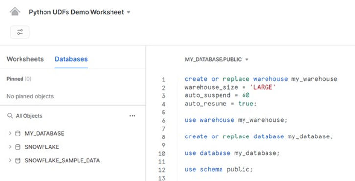
We will start by setting up the environment in our Snowflake trial account, with the creation of a warehouse and a database:
oko
The tweets we are going to analyse are in a JSON file - TweetsChampions.json – which you can download from kaggle directly onto your computer (we placed the file in C:\temp\). We have already used this data in one of our previous blog posts, so we encourage you to look there for further details on how easy it is to analyze semi-structured data in Snowflake. For now, we will create a file format and a stage for this file:
create or replace file format tweets_file_format
type = json;

create or replace stage tweets_stage
file_format = tweets_file_format;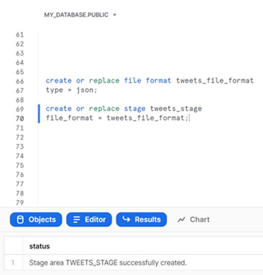
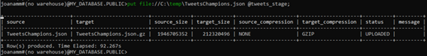
And then use SnowSQL to place the json file in the newly created stage:
use database MY_DATABASE;
put file://C:\temp\TweetsChampions.json @tweets_stage;
We will then run a sequence of SQL commands to create a table that will hold the raw json data, copy the raw data from the json file into this table, then create another table that contains the tweets data in tabular format, and finally inspect a few entries in this table:
create or replace table raw_tweets (tweet variant);

copy into raw_tweets from @tweets_stage;

create or replace table summary_tweets as
	select tweet:user:id::number as user_id,
    tweet:user:followers_count::integer as user_followers_count,
    tweet:id::number as tweet_id,
    tweet:created_at::timestamp as tweet_date,
    tweet:lang::string as tweet_language,
    tweet:text::string as tweet_text
    --,value:text::string as tweet_hashtag_text
    from raw_tweets
    --, lateral flatten(tweet:entities:hashtags)
    where tweet_id is not null and tweet:possibly_sensitive=false
    	and hour(tweet_date)>17;

select * from summary_tweets where tweet_language = 'en' limit 10;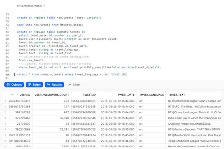
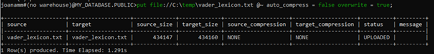
Now that the tweets are in Snowflake, we will set up our sentiment analysis. The nltk package is available to us directly in Snowflake, thanks to the partnership with Anaconda, so we can use it in a similar way to the holidays package in our last blog post. Outside of Snowflake, we would directly use the nltk library to download the VADER analysis model. However, due to Snowflake security constraints, on-demand downloading does not work with Python UDFs. To work around this issue, we will need to download the VADER lexicon locally and provide it to the UDF via a Snowflake stage. We will again use SnowSQL and put the file in the user stage (no need to create a dedicated stage), ensuring it is not compressed:
put file://C:\temp\vader_lexicon.txt @~ auto_compress = false overwrite = true;
We can now create our Python UDF:
create or replace function getSentiment(mySentence string)
returns float
language pythonr
untime_version = 3.8
packages = ('nltk')
imports=('@~/vader_lexicon.txt')
handler = 'getScore'
as $$
import nltk
import sys
IMPORT_DIRECTORY_NAME = "snowflake_import_directory"
import_dir = sys._xoptions[IMPORT_DIRECTORY_NAME]
def getScore(mySentence):
	from nltk.sentiment.vader
    import SentimentIntensityAnalyzer
    lexicon_file = import_dir+'vader_lexicon.txt'
    sentiment_analyzer = SentimentIntensityAnalyzer(lexicon_file)
    sentiment_score = sentiment_analyzer.polarity_scores(mySentence)
['compound']
	return sentiment_score
$$;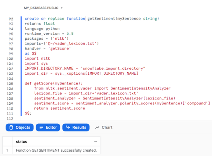
This function will take in a string (which will ultimately be the tweets we want to analyze) and return a float, corresponding to the VADER compound polarity score. As you can see, we use the nltk package and import the VADER lexicon file from our user stage. When we specify the import file, Snowflake copies the staged file to the UDFs import directory in the background. We then need to retrieve the location of this import directory using the sys._xoptions method in our Python code (encased by dollar symbols). Finally, we can define our function and tell nltk to use the VADER lexicon and return a sentiment analysis score.
We can run our function on a simple example:
select getSentiment('I love Argusa!'), getSentiment('I hate the rain');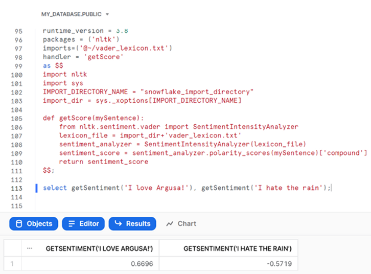
The VADER compound sentiment score runs between -1 (most negative) and 1 (most positive), so our function appears to be working!
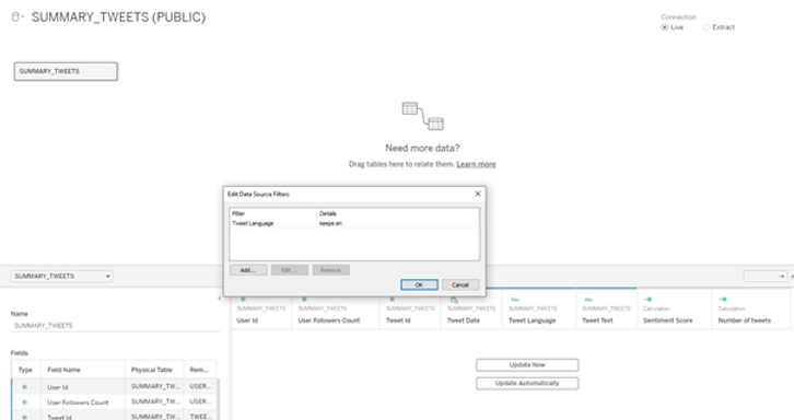
Let us now go to Tableau Desktop and continue our analysis there. We will drag the summary tweets table for analysis and apply a data source filter to focus on English language tweets:
We can then produce a simple visualization of the number of tweets (count distinct of Tweet Id) through time (exact Tweet Date):
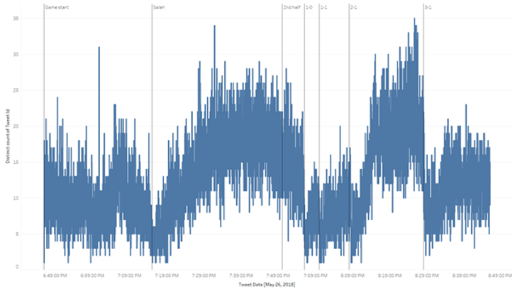
In this example we added a few reference lines indicating significant events throughout the match, to facilitate our analysis. It is interesting to observe, for example, that the number of tweets decreases significantly immediately after a goal is scored.
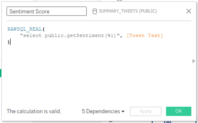
We will now use Tableau’s pass-through functions to run our “getSentiment” Snowflake UDF:
RAWSQL_REAL(
	"select public.getSentiment(%1)", [Tweet Text]
)
We should change the default aggregation of our sentiment score to an average, as it does not make sense to do the default sum on this measure. We can then slightly modify our visualization, by dragging the Sentiment Score calculation to the Color Mark and changing the Tweet Date field to Minute of Tweet Data, instead of the exact date:
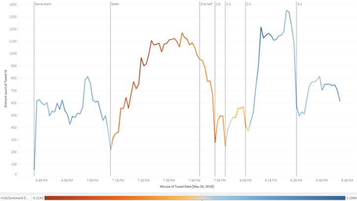
With this new visualization we can see a stable number of tweets being published with, on average, positive sentiments in the first 30 minutes of the game.
At approximately 7:15 PM (second reference line) Liverpool’s player Salah was substituted due to an injury sustained while competing for the ball with Real Madrid’s player Ramos. This event generated angry responses from Salah’s fans, whose insults trended on Twitter. We can see this well in our visualization, as the number of tweets published increases steadily after Salah’s injury, and the average sentiment of the tweets turns negative.
The number of tweets decreased in the second half, but the average sentiment of the tweets remained negative, at least until approximately 8:10 PM, when Real Madrid secured the victory by scoring the second goal. At this point we observe another in increase in the number of tweets and the average sentiment turning positive.
Here is another visualization that shows the average sentiment score of tweets (excluding retweets) mentioning 5 different people involved in the Champions League final:
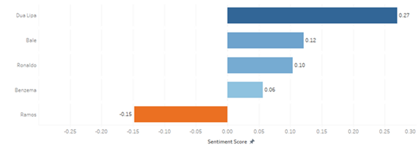
We can see that, of the 5 people analyzed, only Ramos has average negative scores, due to the incident with Salah mentioned previously.
Not all is negative though. The tweets mentioning Dua Lipa, the singer that performed at the opening ceremony, are, on average the most positive of the 5 people analyzed. In fact, the two tweets with the highest sentiment score (0.968 and 0.962) in our dataset are about the performance of the singer:
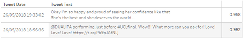
We draw your attention to the fact that these sentiment scores are calculated using complex Python analysis models. But thanks to Snowflake and Tableau it is easy to access these models in familiar environments, and straightforward to produce and analyze results with almost no coding!
In our last blog post - "Running Python in Tableau with Snowflake" - we provided a simple example of how one can leverage the versatility of the Python programming language in Tableau's familiar data visualisation environment, through the usage of Python UDFs (User Defined Functions) available in the Snowflake platform.
In this blog post, we will provide another example of this application, by analyzing tweets captured during the 2018 UEFA Champions League final match. In particular, we will show how to use VADER (Valence Aware Dictionary and Sentiment Reasoner), an open-source sentiment analysis model from the nltk package (Natural Language Tool Kit), to perform sentiment analysis of these tweets.
Similar to our last blog post, if you would like a more hands-on experience and have the possibility of using Tableau, you can set up a Snowflake trial account and follow along with our example.
We will start by setting up the environment in our Snowflake trial account, with the creation of a warehouse and a database:
oko
The tweets we are going to analyse are in a JSON file - TweetsChampions.json – which you can download from kaggle directly onto your computer (we placed the file in C:\temp\). We have already used this data in one of our previous blog posts, so we encourage you to look there for further details on how easy it is to analyze semi-structured data in Snowflake. For now, we will create a file format and a stage for this file:
create or replace file format tweets_file_format
type = json;

create or replace stage tweets_stage
file_format = tweets_file_format;
And then use SnowSQL to place the json file in the newly created stage:
use database MY_DATABASE;
put file://C:\temp\TweetsChampions.json @tweets_stage;
We will then run a sequence of SQL commands to create a table that will hold the raw json data, copy the raw data from the json file into this table, then create another table that contains the tweets data in tabular format, and finally inspect a few entries in this table:
create or replace table raw_tweets (tweet variant);

copy into raw_tweets from @tweets_stage;

create or replace table summary_tweets as
	select tweet:user:id::number as user_id,
    tweet:user:followers_count::integer as user_followers_count,
    tweet:id::number as tweet_id,
    tweet:created_at::timestamp as tweet_date,
    tweet:lang::string as tweet_language,
    tweet:text::string as tweet_text
    --,value:text::string as tweet_hashtag_text
    from raw_tweets
    --, lateral flatten(tweet:entities:hashtags)
    where tweet_id is not null and tweet:possibly_sensitive=false
    	and hour(tweet_date)>17;

select * from summary_tweets where tweet_language = 'en' limit 10;
Now that the tweets are in Snowflake, we will set up our sentiment analysis. The nltk package is available to us directly in Snowflake, thanks to the partnership with Anaconda, so we can use it in a similar way to the holidays package in our last blog post. Outside of Snowflake, we would directly use the nltk library to download the VADER analysis model. However, due to Snowflake security constraints, on-demand downloading does not work with Python UDFs. To work around this issue, we will need to download the VADER lexicon locally and provide it to the UDF via a Snowflake stage. We will again use SnowSQL and put the file in the user stage (no need to create a dedicated stage), ensuring it is not compressed:
put file://C:\temp\vader_lexicon.txt @~ auto_compress = false overwrite = true;
We can now create our Python UDF:
create or replace function getSentiment(mySentence string)
returns float
language pythonr
untime_version = 3.8
packages = ('nltk')
imports=('@~/vader_lexicon.txt')
handler = 'getScore'
as $$
import nltk
import sys
IMPORT_DIRECTORY_NAME = "snowflake_import_directory"
import_dir = sys._xoptions[IMPORT_DIRECTORY_NAME]
def getScore(mySentence):
	from nltk.sentiment.vader
    import SentimentIntensityAnalyzer
    lexicon_file = import_dir+'vader_lexicon.txt'
    sentiment_analyzer = SentimentIntensityAnalyzer(lexicon_file)
    sentiment_score = sentiment_analyzer.polarity_scores(mySentence)
['compound']
	return sentiment_score
$$;
This function will take in a string (which will ultimately be the tweets we want to analyze) and return a float, corresponding to the VADER compound polarity score. As you can see, we use the nltk package and import the VADER lexicon file from our user stage. When we specify the import file, Snowflake copies the staged file to the UDFs import directory in the background. We then need to retrieve the location of this import directory using the sys._xoptions method in our Python code (encased by dollar symbols). Finally, we can define our function and tell nltk to use the VADER lexicon and return a sentiment analysis score.
We can run our function on a simple example:
select getSentiment('I love Argusa!'), getSentiment('I hate the rain');The VADER compound sentiment score runs between -1 (most negative) and 1 (most positive), so our function appears to be working!
Let us now go to Tableau Desktop and continue our analysis there. We will drag the summary tweets table for analysis and apply a data source filter to focus on English language tweets:
We can then produce a simple visualization of the number of tweets (count distinct of Tweet Id) through time (exact Tweet Date):
In this example we added a few reference lines indicating significant events throughout the match, to facilitate our analysis. It is interesting to observe, for example, that the number of tweets decreases significantly immediately after a goal is scored.
We will now use Tableau’s pass-through functions to run our “getSentiment” Snowflake UDF:
RAWSQL_REAL(
	"select public.getSentiment(%1)", [Tweet Text]
)
We should change the default aggregation of our sentiment score to an average, as it does not make sense to do the default sum on this measure. We can then slightly modify our visualization, by dragging the Sentiment Score calculation to the Color Mark and changing the Tweet Date field to Minute of Tweet Data, instead of the exact date:
With this new visualization we can see a stable number of tweets being published with, on average, positive sentiments in the first 30 minutes of the game.
At approximately 7:15 PM (second reference line) Liverpool’s player Salah was substituted due to an injury sustained while competing for the ball with Real Madrid’s player Ramos. This event generated angry responses from Salah’s fans, whose insults trended on Twitter. We can see this well in our visualization, as the number of tweets published increases steadily after Salah’s injury, and the average sentiment of the tweets turns negative.
The number of tweets decreased in the second half, but the average sentiment of the tweets remained negative, at least until approximately 8:10 PM, when Real Madrid secured the victory by scoring the second goal. At this point we observe another in increase in the number of tweets and the average sentiment turning positive.
Here is another visualization that shows the average sentiment score of tweets (excluding retweets) mentioning 5 different people involved in the Champions League final:
We can see that, of the 5 people analyzed, only Ramos has average negative scores, due to the incident with Salah mentioned previously.
Not all is negative though. The tweets mentioning Dua Lipa, the singer that performed at the opening ceremony, are, on average the most positive of the 5 people analyzed. In fact, the two tweets with the highest sentiment score (0.968 and 0.962) in our dataset are about the performance of the singer:
We draw your attention to the fact that these sentiment scores are calculated using complex Python analysis models. But thanks to Snowflake and Tableau it is easy to access these models in familiar environments, and straightforward to produce and analyze results with almost no coding!