From JSON to insight with Snowflake

Snowflake is a unique integrated data platform, conceived from the ground up for the cloud. Its patented multi-cluster, shared-data architecture features compute, storage and cloud services layers that scale independently, enabling any user to work with any data, with no limits on scale, performance or flexibility.


Snowflake supports modern data warehouses, augmented data lakes, advanced data science, intensive application development, secure data exchanges and integrated data engineering, all in one place, enabling data and BI professionals to make the most of their data. More important, Snowflake is secure and governed by design, and is delivered as a service with near-zero maintenance.
The Snowflake data cloud offers some truly powerful features. For example, its management of metadata allows for zero-copy cloning and time-travel. The compute layer can scale up and out at any time to handle complex and concurrent workloads, and you only pay for what you use. Furthermore, storage and compute are kept separate, ensuring anyone can access data without running into contention issues.
One of Snowflake’s most compelling features is its native support for semi-structured data. With Snowflake there is no need to implement separate systems to process structured and semi-structured data, which is crucial in the current times of Big Data and IoT. The process of loading a CSV or a JSON file is identical and seamless. Furthermore, Snowflake is a SQL platform so you can query both structured and semi-structured data using SQL with similar performance, no need to learn new programming skills.
Here we will show, using a simple example, how easy it is to load, query and analyze semi-structured data in Snowflake. We will specifically be looking into data from Twitter. This is particularly interesting given the volume of data produced by Twitter, and the fact that Twitter’s data model relies on semi-structured data, as tweets are typically encoded using JSON.
Follow along
If you would like a more hands-on experience, you can set up your own Snowflake account and follow along with our example by copying and pasting the code. Please visit Snowflake here to sign up for a free trial. Because Snowflake is delivered as a service all you need to do is choose an edition of Snowflake - we recommend Entreprise - and a cloud platform/region – AWS, Azure or GCP (Snowflake is cloud agnostic, so your experience will be similar regardless of the platform you choose).
We will be playing with a JSON dataset containing tweets captured during the 2018 UEFA Champions League final match. You can download the JSON file - TweetsChampions.json - directly onto your computer from kaggle. Due to file size restrictions, we will be using SnowSQL, Snowflake’s command line client, to load the data from our computer into Snowflake. To install SnowSQL please visit Snowflake’s Repository.
Loading
Let us start by setting things up. Below you can see a screenshot of the Snowflake web UI. This is an extremely powerful tool and can be used to perform nearly any task in Snowflake. Here we will use the Worksheets specifically, to create and submit SQL queries and operations. Notice how the SQL results appear at the bottom of the page. Keep in mind most of these operations can be executed using other features of the web interface that do not require writing SQL.
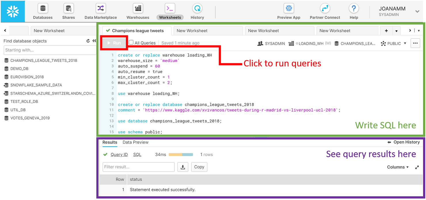
We started by creating a medium-sized warehouse named “LOADING_WH”. Warehouses in Snowflake are virtual computing units that provide compute power to execute queries. This warehouse consists of a cluster of 4 servers. We have set max_cluster_count = 2, which means that we allow Snowflake to automatically add another cluster to the virtual warehouse, to help improve performance in case multiple queries are submitted concurrently. Remember that with Snowflake you only pay for compute when warehouses are running. We therefore set our LOADING_WH to auto-suspend within 60 seconds of inactivity. To simplify our workload, we used the auto_resume = true option as well, which will automatically fire up the warehouse once a query is submitted. The operation use warehouse loading_WH indicates that queries submitted in the worksheet will use this warehouse for computing power.
CREATE OR REPLACE WAREHOUSE loading_WH
WAREHOUSE_SIZE = 'medium'
AUTO_SUSPEND = 60
AUTO_RESUME = true
MIN_CLUSTER_COUNT = 1
MAX_CLUSTER_COUNT = 2;

USE WAREHOUSE loading_WH;
We also created a CHAMPIONS_LEAGUE_TWEETS_2018 database to hold our data, and we opted to use the PUBLIC schema automatically created within that database for simplicity. We also indicated that we will be using those database and schema in the context of the worksheet.
CREATE OR REPLACE DATABASE champions_league_tweets_2018
COMMENT = 'https://www.kaggle.com/xvivancos/tweets-during-r-madrid-vs-liverpool-ucl-2018';

USE DATABASE champions_league_tweets_2018;

USE SCHEMA public;
To load data into Snowflake you generally need to follow these steps:
- Create a file format, to inform Snowflake of what kind of data you will be loading. Snowflake supports loading of both structured (CSV, TSV, ...) and semi-structured (JSON, Avro, ORC, Parquet and XML) data. Here we simply created a file format object for JSON files named TWEETS_FILE_FORMAT.
CREATE OR REPLACE FILE_FORMAT tweets_file_format
TYPE = json;- Create a so-called stage. A stage is an intermediate area where you will put your data files before loading them into tables. Stages in Snowflake can be internal (they exist within Snowflake) or external (e.g. an AWS S3 bucket). For this example, we created an internal stage called TWEETS_STAGE. We also referenced the previously created file format in the stage definition, since the stage will hold JSON files. We then used SnowSQL to put our JSON data file into this internal stage. Once the data is placed into the stage, you can list its contents. In the screenshot below you will find the output of the list command. Notice how the JSON file is compressed – this is standard in Snowflake and is done automatically.
CREATE OR REPLACE STAGE tweets_stage
FILE_FORMAT = tweets_file_format;

//use SnowSQL to run the put command and stage local json file
//put file://C:\temp\TweetsChampions.json @tweets_stage;

LIST @tweets_stage;- Create a table to hold your data. Semi-structured data in particular is loaded into tables with a single column of type VARIANT. This is an innovative and flexible data type developed by Snowflake, specifically to hold a variety of semi-structured data.
CREATE OR REPLACE TABLE raw_tweets (tweet variant);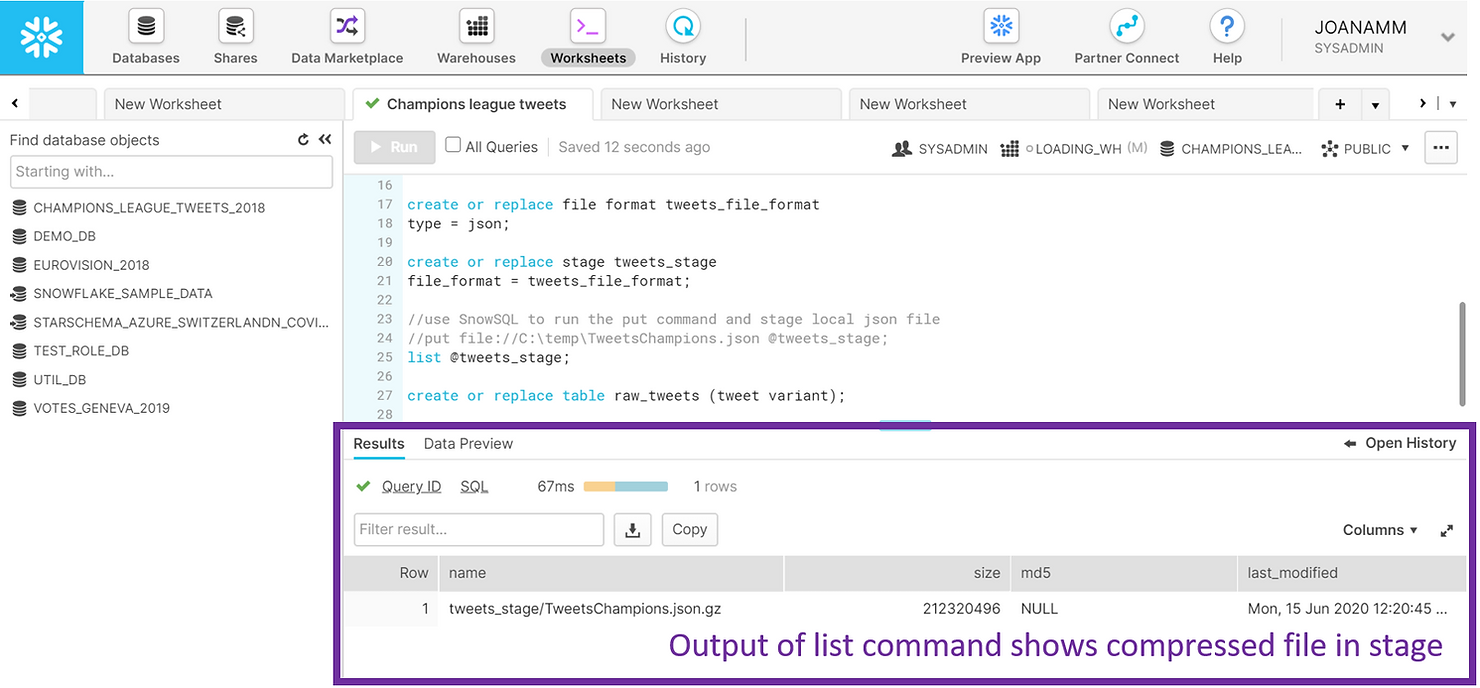
Everything is now in place for us to load the data, and we simply need to copy from the stage into the table. Snowflake knows how to parse and identify the structure in the JSON file, so in a little over a minute we were able to fill our RAW_TWEETS table with approximately 350 thousand rows – 1 row per tweet.
COPY INTO raw_tweets FROM @tweets_stage;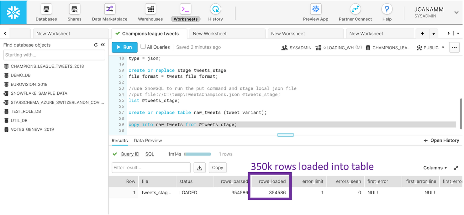
Querying
Now that the data has been loaded, we can run a simple SELECT statement on the RAW_TWEETS table, and explore what each of the rows looks like by clicking it in the results panel in the web UI.
SELECT tweet FROM raw_tweets LIMIT 3;
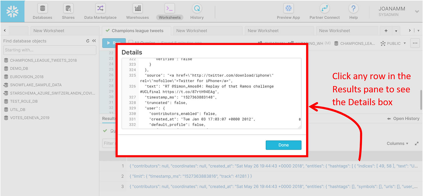
The JSON tweet is made up of multiple nested entities, each with different key-value pairs. Looking at these in the screenshot above may seem daunting, but navigating JSON data in Snowflake is actually simple – we just have to create paths using colons. In the example below, we retrieve the user ID of the first 10 tweets.
SELECT tweet:user:id AS user_id FROM raw_tweets
LIMIT 10;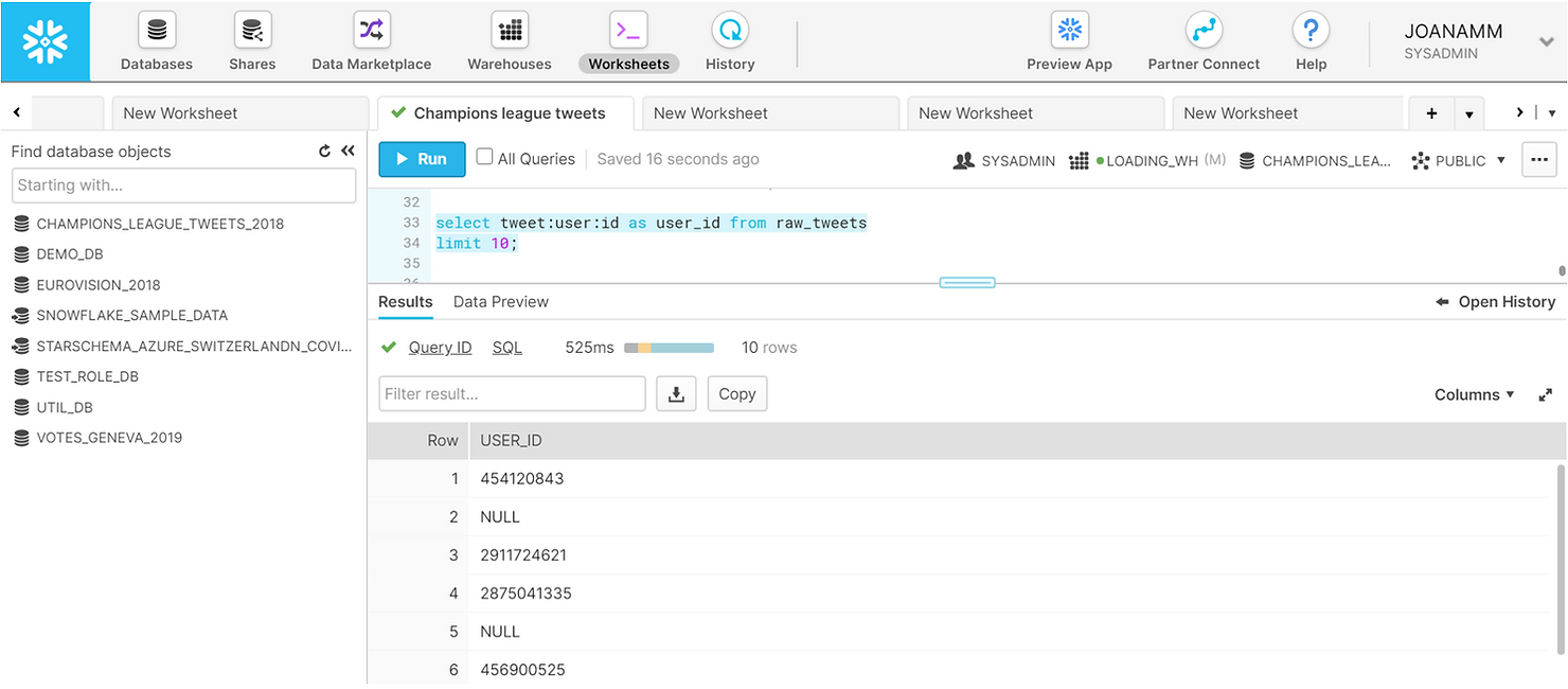
We can easily retrieve more information from the tweets and get a familiar structured and tabular preview of the data in the results pane.
SELECT tweet:user:id AS user_id,
	tweet:user:followers_count AS user_followers_count,
    tweet:id AS tweet_id,
    tweet:created_at AS tweet_date,
    tweet:lang AS tweet_language,
    tweet:text AS tweet_text,
    tweet:entities:hashtags AS tweet_hashtags
FROM raw_tweets
LIMIT 10;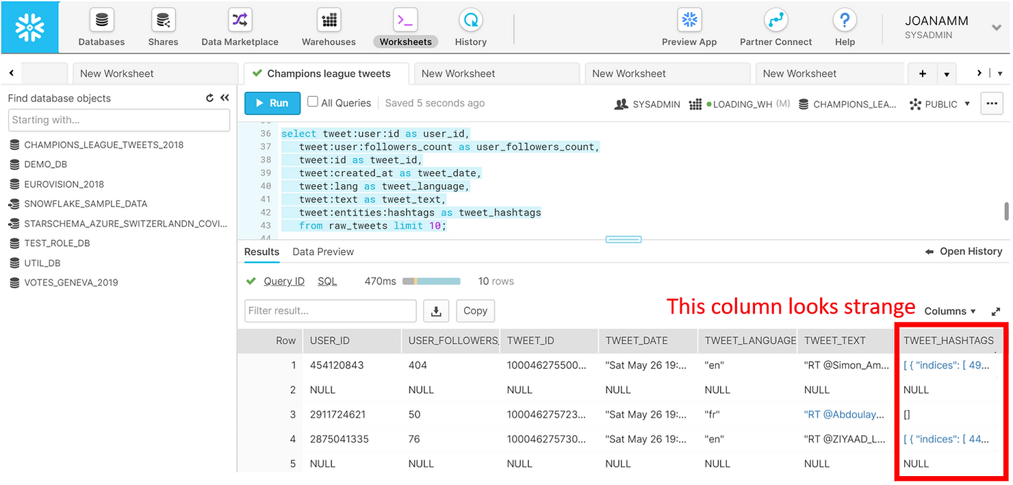
Notice the last column holding the hashtags though. We can click it in the results pane to explore the details further.
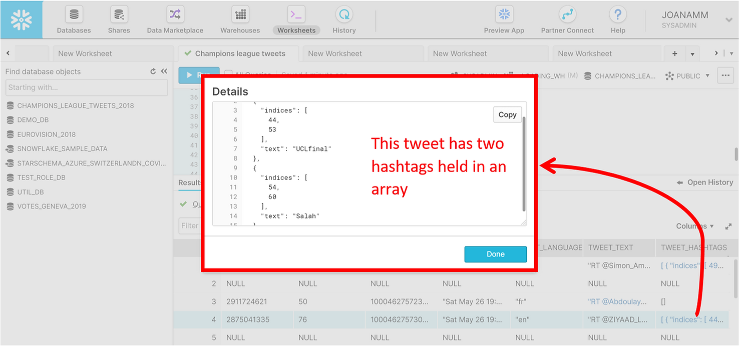
A single tweet can have multiple hashtags, and these are actually held in arrays. To see all the hashtags in a tweet in a tabular format we need to flatten the data. Once again, this is a simple operation in Snowflake. You can see below a preview of the first 10 hashtags in the dataset. Notice how the same tweet can have multiple hashtags. Now each row in the results pane is no longer a single tweet, but rather a hashtag.
SELECT tweet:id AS tweet_id,
	value:text AS tweet_hashtag_text
FROM raw_tweets,
LATERAL FLATTEN(tweet:entities:hashtags)
LIMIT 10;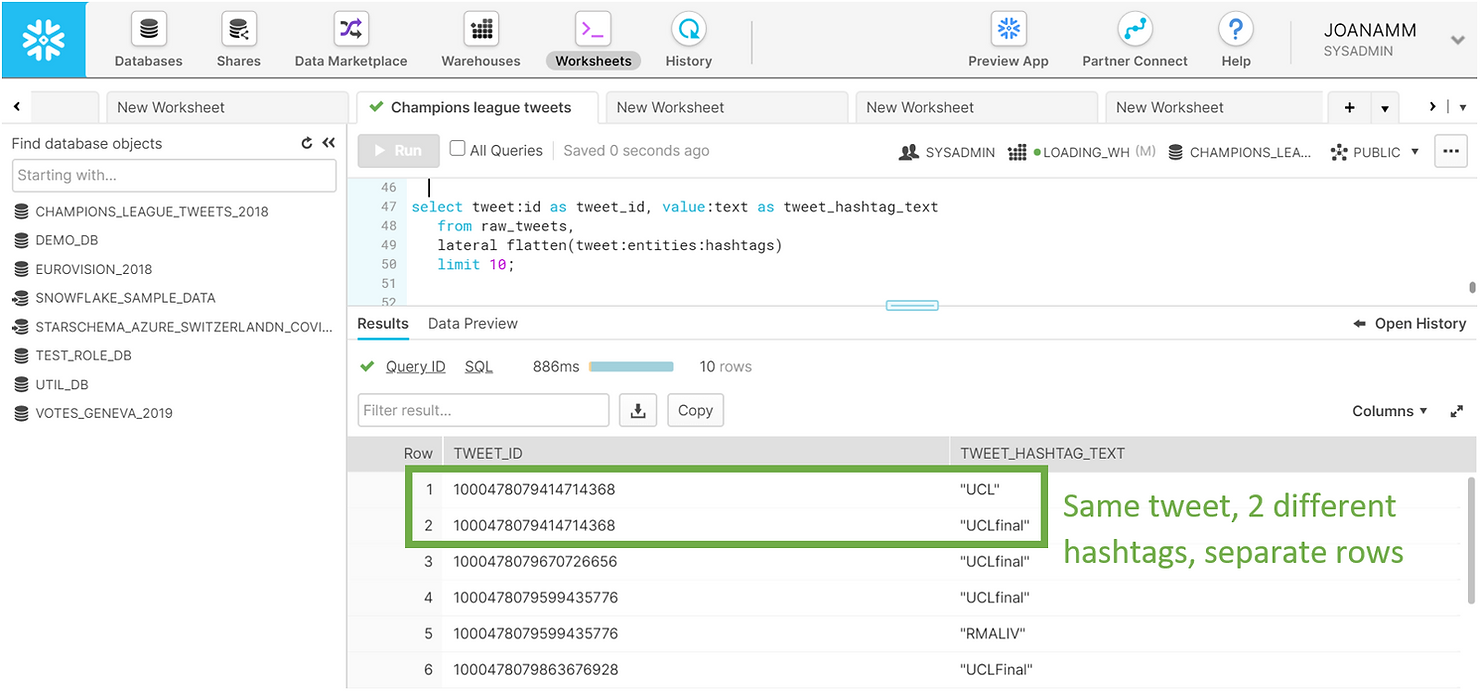
As we showed, Snowflake allows you to use simple SQL statements to query a complex JSON dataset. To optimize the analysis process ahead let us save the results of these queries in a view. Compared to the other queries shown above we have simply cast the columns into the appropriate data types and filtered out potentially sensitive data.
CREATE OR REPLACE view summary_tweets AS
	SELECT tweet:user:id::number AS user_id,
		tweet:user:followers_count::integer AS user_followers_count,
		tweet:id::number AS tweet_id,
		tweet:created_at::timestamp AS tweet_date,
		tweet:lang::string AS tweet_language,
		tweet:text::string AS tweet_text,
		value:text::string AS tweet_hashtag_text from raw_tweets,
	LATERAL FLATTEN(tweet:entities:hashtags)
	WHERE tweet_id IS NOT NULL AND tweet:possibly_sensitive=FALSE AND hour(tweet_date)>17;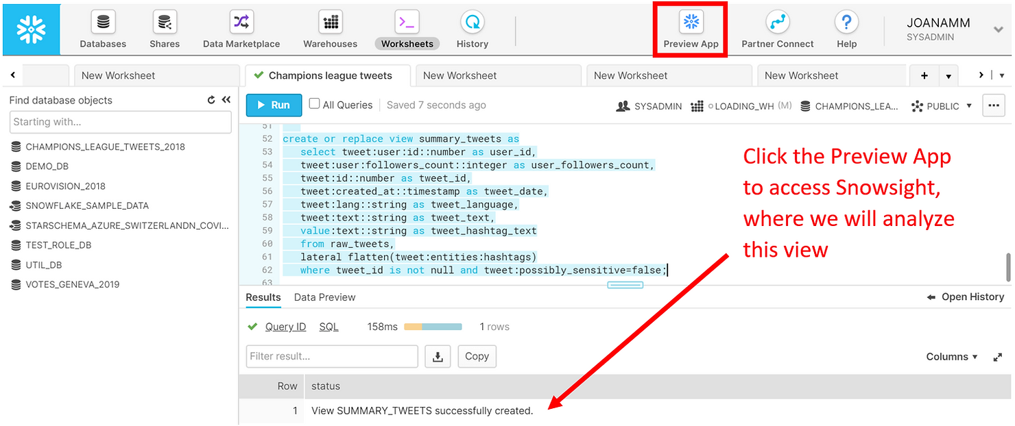
Analyzing
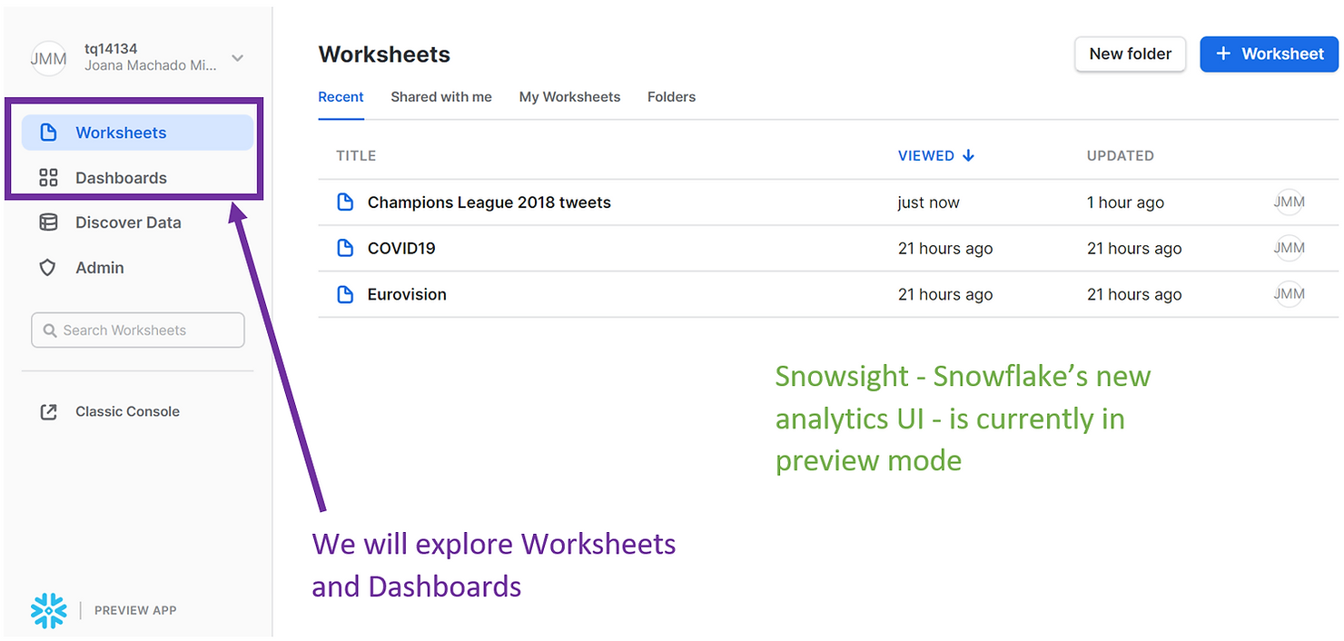
To analyze our tweets we will use Snowsight, Snowflake’s new analytics UI. Snowsight is still in preview mode, but it can currently be accessed from the Preview App at the top of the web UI. We will be using the Worksheets, as well as the new Dashboards feature of Snowsight.
If you open a new Worksheet in Snowsight, you might find that, apart from a design change, they are very similar to the classic Worksheets used above. For example, we can run SQL statements just like before, but we do have the added benefit of auto-completion. Here we are selecting all the hashtags from the SUMMARY_TWEETS view we previously created, and the results of our query also appear in the Results pane at the bottom.
SELECT UPPER(tweet_hashtag_text) FROM summary_tweets;

However, a powerful feature of the brand new Snowsight unlocks once we click on Chart.
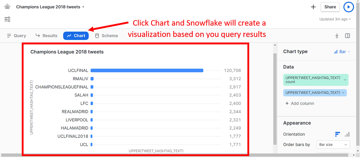
As you can see, Snowflake automatically produced a visualization showing the frequency of each hashtag in our results, allowing us to see much more than what the Results pane had to offer. The hashtag UCLFINAL was used the most often - 120 thousand times. Other popular hashtags reference the teams that played in the finals, namely Real Madrid and Liverpool.
Here is another simple example, of a bar chart of the number of tweets by user. You can use the pane on the right to modify and format the charts if you wish.
SELECT user_id,
	COUNT(distinct tweet_id) AS tweet_count
FROM summary_tweets
GROUP BY 1
ORDER BY tweet_count DESC
LIMIT 10;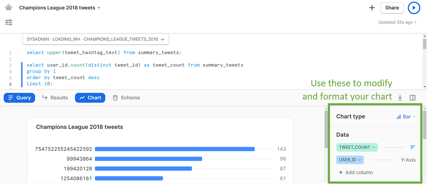
Or yet another example, this time a line chart, showing when the different tweets were created.
SELECT tweet_date,
	COUNT(DISTINCT tweet_id) AS tweet_count
FROM summary_tweets
GROUP BY tweet_date;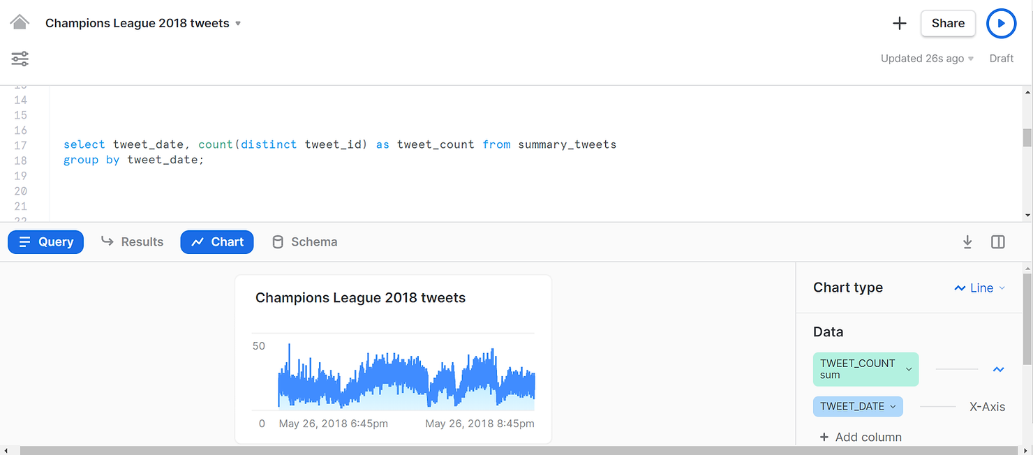
And with a few more clicks in Snowsight, we can create a dashboard to summarize our findings, all within Snowflake!
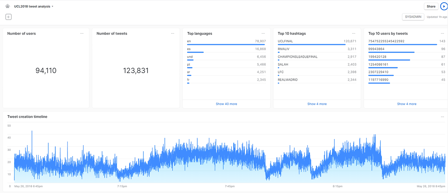
In summary, Snowflake is a unique data platform that unlocks the unlimited resources of the cloud and enables companies to become data-driven in a modern data world. We hope we were able to show you how quickly and easily you can go from a confusing semi-structured dataset to an analytics dashboard, all within Snowflake. If you are curious about Snowflake reach out to Team Argusa at info@argusa.ch.
Snowflake is a unique integrated data platform, conceived from the ground up for the cloud. Its patented multi-cluster, shared-data architecture features compute, storage and cloud services layers that scale independently, enabling any user to work with any data, with no limits on scale, performance or flexibility.
Snowflake supports modern data warehouses, augmented data lakes, advanced data science, intensive application development, secure data exchanges and integrated data engineering, all in one place, enabling data and BI professionals to make the most of their data. More important, Snowflake is secure and governed by design, and is delivered as a service with near-zero maintenance.
The Snowflake data cloud offers some truly powerful features. For example, its management of metadata allows for zero-copy cloning and time-travel. The compute layer can scale up and out at any time to handle complex and concurrent workloads, and you only pay for what you use. Furthermore, storage and compute are kept separate, ensuring anyone can access data without running into contention issues.
One of Snowflake’s most compelling features is its native support for semi-structured data. With Snowflake there is no need to implement separate systems to process structured and semi-structured data, which is crucial in the current times of Big Data and IoT. The process of loading a CSV or a JSON file is identical and seamless. Furthermore, Snowflake is a SQL platform so you can query both structured and semi-structured data using SQL with similar performance, no need to learn new programming skills.
Here we will show, using a simple example, how easy it is to load, query and analyze semi-structured data in Snowflake. We will specifically be looking into data from Twitter. This is particularly interesting given the volume of data produced by Twitter, and the fact that Twitter’s data model relies on semi-structured data, as tweets are typically encoded using JSON.
Follow along
If you would like a more hands-on experience, you can set up your own Snowflake account and follow along with our example by copying and pasting the code. Please visit Snowflake here to sign up for a free trial. Because Snowflake is delivered as a service all you need to do is choose an edition of Snowflake - we recommend Entreprise - and a cloud platform/region – AWS, Azure or GCP (Snowflake is cloud agnostic, so your experience will be similar regardless of the platform you choose).
We will be playing with a JSON dataset containing tweets captured during the 2018 UEFA Champions League final match. You can download the JSON file - TweetsChampions.json - directly onto your computer from kaggle. Due to file size restrictions, we will be using SnowSQL, Snowflake’s command line client, to load the data from our computer into Snowflake. To install SnowSQL please visit Snowflake’s Repository.
Loading
Let us start by setting things up. Below you can see a screenshot of the Snowflake web UI. This is an extremely powerful tool and can be used to perform nearly any task in Snowflake. Here we will use the Worksheets specifically, to create and submit SQL queries and operations. Notice how the SQL results appear at the bottom of the page. Keep in mind most of these operations can be executed using other features of the web interface that do not require writing SQL.
We started by creating a medium-sized warehouse named “LOADING_WH”. Warehouses in Snowflake are virtual computing units that provide compute power to execute queries. This warehouse consists of a cluster of 4 servers. We have set max_cluster_count = 2, which means that we allow Snowflake to automatically add another cluster to the virtual warehouse, to help improve performance in case multiple queries are submitted concurrently. Remember that with Snowflake you only pay for compute when warehouses are running. We therefore set our LOADING_WH to auto-suspend within 60 seconds of inactivity. To simplify our workload, we used the auto_resume = true option as well, which will automatically fire up the warehouse once a query is submitted. The operation use warehouse loading_WH indicates that queries submitted in the worksheet will use this warehouse for computing power.
CREATE OR REPLACE WAREHOUSE loading_WH
WAREHOUSE_SIZE = 'medium'
AUTO_SUSPEND = 60
AUTO_RESUME = true
MIN_CLUSTER_COUNT = 1
MAX_CLUSTER_COUNT = 2;

USE WAREHOUSE loading_WH;
We also created a CHAMPIONS_LEAGUE_TWEETS_2018 database to hold our data, and we opted to use the PUBLIC schema automatically created within that database for simplicity. We also indicated that we will be using those database and schema in the context of the worksheet.
CREATE OR REPLACE DATABASE champions_league_tweets_2018
COMMENT = 'https://www.kaggle.com/xvivancos/tweets-during-r-madrid-vs-liverpool-ucl-2018';

USE DATABASE champions_league_tweets_2018;

USE SCHEMA public;
To load data into Snowflake you generally need to follow these steps:
- Create a file format, to inform Snowflake of what kind of data you will be loading. Snowflake supports loading of both structured (CSV, TSV, ...) and semi-structured (JSON, Avro, ORC, Parquet and XML) data. Here we simply created a file format object for JSON files named TWEETS_FILE_FORMAT.
CREATE OR REPLACE FILE_FORMAT tweets_file_format
TYPE = json;- Create a so-called stage. A stage is an intermediate area where you will put your data files before loading them into tables. Stages in Snowflake can be internal (they exist within Snowflake) or external (e.g. an AWS S3 bucket). For this example, we created an internal stage called TWEETS_STAGE. We also referenced the previously created file format in the stage definition, since the stage will hold JSON files. We then used SnowSQL to put our JSON data file into this internal stage. Once the data is placed into the stage, you can list its contents. In the screenshot below you will find the output of the list command. Notice how the JSON file is compressed – this is standard in Snowflake and is done automatically.
CREATE OR REPLACE STAGE tweets_stage
FILE_FORMAT = tweets_file_format;

//use SnowSQL to run the put command and stage local json file
//put file://C:\temp\TweetsChampions.json @tweets_stage;

LIST @tweets_stage;- Create a table to hold your data. Semi-structured data in particular is loaded into tables with a single column of type VARIANT. This is an innovative and flexible data type developed by Snowflake, specifically to hold a variety of semi-structured data.
CREATE OR REPLACE TABLE raw_tweets (tweet variant);Everything is now in place for us to load the data, and we simply need to copy from the stage into the table. Snowflake knows how to parse and identify the structure in the JSON file, so in a little over a minute we were able to fill our RAW_TWEETS table with approximately 350 thousand rows – 1 row per tweet.
COPY INTO raw_tweets FROM @tweets_stage;
Querying
Now that the data has been loaded, we can run a simple SELECT statement on the RAW_TWEETS table, and explore what each of the rows looks like by clicking it in the results panel in the web UI.
SELECT tweet FROM raw_tweets LIMIT 3;
The JSON tweet is made up of multiple nested entities, each with different key-value pairs. Looking at these in the screenshot above may seem daunting, but navigating JSON data in Snowflake is actually simple – we just have to create paths using colons. In the example below, we retrieve the user ID of the first 10 tweets.
SELECT tweet:user:id AS user_id FROM raw_tweets
LIMIT 10;
We can easily retrieve more information from the tweets and get a familiar structured and tabular preview of the data in the results pane.
SELECT tweet:user:id AS user_id,
	tweet:user:followers_count AS user_followers_count,
    tweet:id AS tweet_id,
    tweet:created_at AS tweet_date,
    tweet:lang AS tweet_language,
    tweet:text AS tweet_text,
    tweet:entities:hashtags AS tweet_hashtags
FROM raw_tweets
LIMIT 10;
Notice the last column holding the hashtags though. We can click it in the results pane to explore the details further.
A single tweet can have multiple hashtags, and these are actually held in arrays. To see all the hashtags in a tweet in a tabular format we need to flatten the data. Once again, this is a simple operation in Snowflake. You can see below a preview of the first 10 hashtags in the dataset. Notice how the same tweet can have multiple hashtags. Now each row in the results pane is no longer a single tweet, but rather a hashtag.
SELECT tweet:id AS tweet_id,
	value:text AS tweet_hashtag_text
FROM raw_tweets,
LATERAL FLATTEN(tweet:entities:hashtags)
LIMIT 10;
As we showed, Snowflake allows you to use simple SQL statements to query a complex JSON dataset. To optimize the analysis process ahead let us save the results of these queries in a view. Compared to the other queries shown above we have simply cast the columns into the appropriate data types and filtered out potentially sensitive data.
CREATE OR REPLACE view summary_tweets AS
	SELECT tweet:user:id::number AS user_id,
		tweet:user:followers_count::integer AS user_followers_count,
		tweet:id::number AS tweet_id,
		tweet:created_at::timestamp AS tweet_date,
		tweet:lang::string AS tweet_language,
		tweet:text::string AS tweet_text,
		value:text::string AS tweet_hashtag_text from raw_tweets,
	LATERAL FLATTEN(tweet:entities:hashtags)
	WHERE tweet_id IS NOT NULL AND tweet:possibly_sensitive=FALSE AND hour(tweet_date)>17;
Analyzing
To analyze our tweets we will use Snowsight, Snowflake’s new analytics UI. Snowsight is still in preview mode, but it can currently be accessed from the Preview App at the top of the web UI. We will be using the Worksheets, as well as the new Dashboards feature of Snowsight.
If you open a new Worksheet in Snowsight, you might find that, apart from a design change, they are very similar to the classic Worksheets used above. For example, we can run SQL statements just like before, but we do have the added benefit of auto-completion. Here we are selecting all the hashtags from the SUMMARY_TWEETS view we previously created, and the results of our query also appear in the Results pane at the bottom.
SELECT UPPER(tweet_hashtag_text) FROM summary_tweets;
However, a powerful feature of the brand new Snowsight unlocks once we click on Chart.
As you can see, Snowflake automatically produced a visualization showing the frequency of each hashtag in our results, allowing us to see much more than what the Results pane had to offer. The hashtag UCLFINAL was used the most often - 120 thousand times. Other popular hashtags reference the teams that played in the finals, namely Real Madrid and Liverpool.
Here is another simple example, of a bar chart of the number of tweets by user. You can use the pane on the right to modify and format the charts if you wish.
SELECT user_id,
	COUNT(distinct tweet_id) AS tweet_count
FROM summary_tweets
GROUP BY 1
ORDER BY tweet_count DESC
LIMIT 10;
Or yet another example, this time a line chart, showing when the different tweets were created.
SELECT tweet_date,
	COUNT(DISTINCT tweet_id) AS tweet_count
FROM summary_tweets
GROUP BY tweet_date;
And with a few more clicks in Snowsight, we can create a dashboard to summarize our findings, all within Snowflake!
In summary, Snowflake is a unique data platform that unlocks the unlimited resources of the cloud and enables companies to become data-driven in a modern data world. We hope we were able to show you how quickly and easily you can go from a confusing semi-structured dataset to an analytics dashboard, all within Snowflake. If you are curious about Snowflake reach out to Team Argusa at info@argusa.ch.