Tracking time changes in dimensional modelling with WhereScape
In the data warehousing world dimensional modelling is one of the simplest and most straightforward ways to present data to users. This modelling type divides data into facts, mostly quantitative data that represent measures at specific points in time, and dimensions, qualitative attributes that describe the context in which the measures are taken. For example, in the event “a car was sold in Germany for 20000 euros” the “20000 euros” is a fact and “Germany” is an attribute (therefore a dimension).
This article specifically deals with different ways to treat changing attributes with time. This might include products changing name, people changing address and so on.
The book “The data Warehouse Toolkit”, by R. Kimball and M. Ross, describes in detail eight methods to track time changes in dimensional modelling. Here we will discuss a subset of those methods, using the notation introduced by the authors in the book.
Type 0: Keep original
This method is the simplest and it is suited to treat any field with “original” (or equivalent) in its name. These values are simply not allowed to be changed. If a new value is found it is discarded and the original value is kept.
Type 1: Overwrite
This method is suited for changes that are linked to errors or for dealing with fields for which the business is not interested in tracking time changes. The method consists in overwriting the previous value. One example is customers changing birthday dates. The birthday for a person normally cannot change so we can safely assume that, if it does change, it is due to a typing mistake. For this reason, we will discard the previous birthday date and keep always the latest value. This is opposite of the type 0 approach.
Type 2: Add new row
Here we actually start tracking changes. The Type 2 method adds a new row to the dimension. New facts will be linked to the new key and old facts will keep being linked to the old key. A use case for this approach would be changing addresses. For analytical purposes, we would want to keep the address information from which each sale was made. Otherwise we might see changes in measures, e.g. delivery time, that would not be explicable if we replace the address also for old sales (which would be Type 1).
In this method some attributes need to be added on each row of the dimension. Attribute 1 and 2 are compulsory and the others are optional:
- Start date: date from which the record is valid
- End date: date up to which the record is valid
- Current flag: This flags the currently active entry, for easy filtering
- Change date: The date when the change was recorded in the data warehouse which could be different from the date that customer changed their address
- Change reason: To track which attribute on a dimension caused the creation of a new line.
Type 3: Add new column (or alternate reality)
This method is useful when a fundamental change happens in the way an attribute is defined, and the business wants to track the attribute in its old and new definition. A typical example is changes in product categorisation following a merger with another society. A TV set could be previously categorised under “electronics” and be categorised under “media” in the new company. Analysts want to be able to choose which categorisation to consider. In this case a new column is added to the dimensions mapping the old value to the new value.
Type 4: Add Mini-dimension
Sometimes in a dimension there are attributes that change at different speeds. For example, in a customer dimension, there could be the address that changes normally every few years, and the current preferred delivery method, that could change even every day as it is often modifiable with a simple click on a website. Tracking this attribute using the Type 2 approach may cause the number of rows in the dimension to grow rapidly making queries on slow changing parameters less performant. The solution is to split the customer dimension in two, each one with its own primary key in the fact table separately. One will track slow changing attributes and the other one rapidly changing ones.
Type 5: Add mini dimension and type 1 outrigger
This method is similar to Type 4 but in addition it includes the primary key of the rapidly changing dimension as a foreign key to the “main” dimension table, i.e. the table containing the slowly changing dimension. This allows to link the two dimensions directly without going through a fact table. On the other hand, the ‘main’ dimension table can only contain the “current” version of the rapidly changing attribute.
Automate it all using WhereScape
All this looks complicated to implement writing explicit SQL? There is a solution for you. Luckily these methods are based on simple rules, so they lend themselves easily to automation! WhereScape is a leader with 20 years’ experience in Data Warehouse automation. While using WhereScape, you choose the type of change tracking you want, and a wizard will help you configure the implementation without having to write a single a line of code. Furthermore, this work is easily reusable for several dimensions. In the case you want to diverge from the standard rules defined by Kimball, it is possible to edit and customise the template which generates the code, and thus automate the creation of your own change tracking algorithm.
Now, let’s see how it works. For the following example, we will suppose data is already loaded in the target database into a stage table containing markets information, including their location and characteristics.
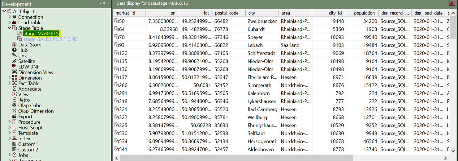
Stage tables are working tables where transformations are done on data before loading it to the final objects (dimensions or fact tables). Typically stage tables are temporary and truncated at every load cycle. This stage table could be sourcing several source tables and already implement complex business logic. This is a good topic for another article. For now, we will focus on how to build a Type 2 Slowly Changing Dimension out of this stage table.
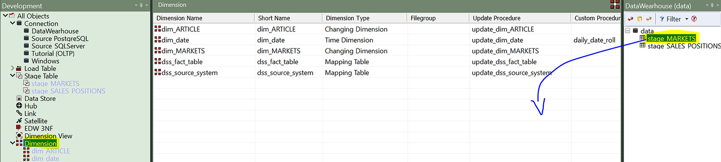
All we have to do is click on the “Dimension” element type in the left pane and then drag and drop the stage table into the work area.
A wizard will pop-up, helping you to configure your new dimension.
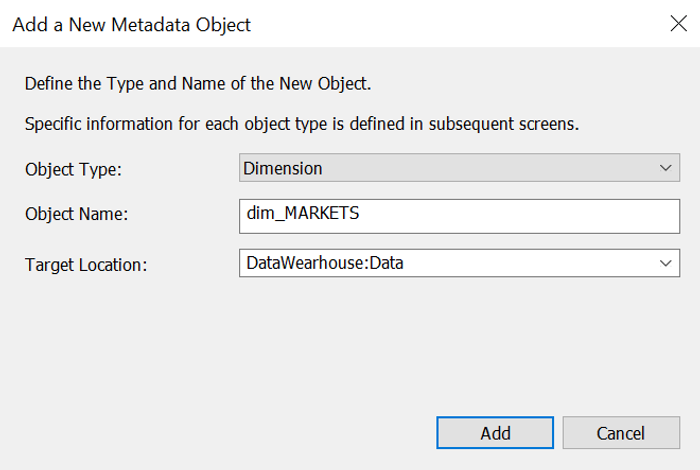
First, we need to give it a name. Notice that the wizard proposes a name for this table, following data warehouse best practices: it uses the name of the stage table and replaces “stage” with “dim”. You can of course customise the naming convention as well as a single entity name that you do not want to follow the convention. In addition, you can decide in what location to store your dimension. For example, permanently stored entities (as dimensions) are typically stored in a location with more robust backup features.
The second window asks you what kind of dimensions you want to build. As you can see Type 1, 2 and 3 are possible. You can also choose to use system generated timestamps or data driven ones. For this example, we will choose “Slowly Changing” (Type 2).

The next window will allow you to fully document your dimension, including its grain, purpose and usage. All this information will appear in the automatically produced documentation.
Most importantly, the wizard will build the code that will manage the inserts and updates. Modifying the DDL (data definition language) is also possible if necessary. In order to customise the update procedure, click on “Rebuild”.
In the next window you can choose to “Create” or “Create and Load”. The reason is that this might be a large table and the load can take a long time. You can therefore conveniently decide not to load the dimensions immediately after creation but later, in the background, via a scheduler.
In the following window you are asked to configure the business key, i.e. the field that identifies a business element. It could be a client, a product or in this case a market. We will choose “market_id”. At the bottom of this window, you will find a helpful description of the element you are currently editing.
We have the possibility to setup all sorts of options, but the defaults work well in most of the use cases. The last step is deciding on which attributes we want to track change. You can do that under the “Change Detection” section.
The choice is up to you and your business representatives. For this example, we will choose population and area. A market represents a specific location, so its longitude and latitude do not change as well as the name of the city it is in. If they do change this is probably due to a mistake so we do not want to track this change in time. On the other hand, population and area are measured every year and in fast developing areas may change rapidly. And it can be interesting to keep track of how the context was when old sales were made. We will therefore track change on these two attributes.
Now we click on “OK” and our dimension is ready.
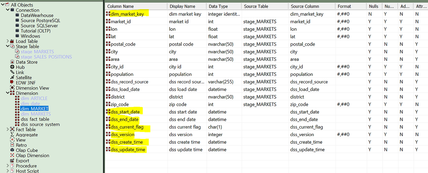
Note that a few fields were automatically created. These include the numeric surrogate key to be used as a foreign key in the fact table and all change attributes: start and end validity dates, current flag, version, first create time and last update times. As the data warehouse evolves, these fields will manage themselves thanks to the predefined update procedure that you configured using the wizard.
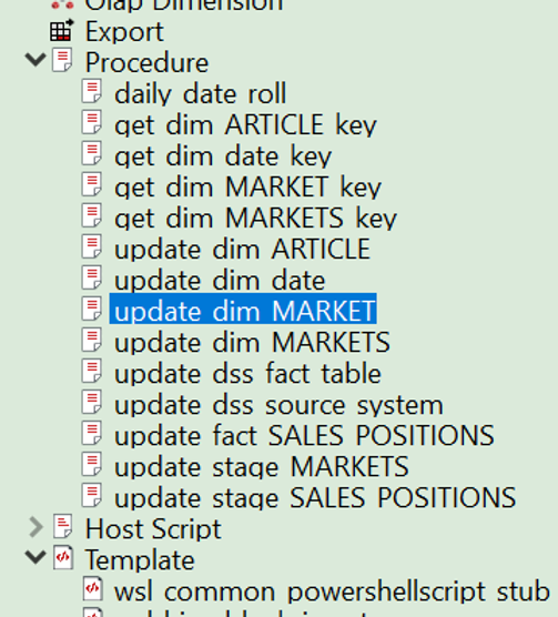
Looking under “Procedures” we are able to inspect the generated code and modify it, if needed. Under “Templates” it is also possible to modify the template that generates the code, in a way that all future dimensions will be built with our customisations.
WhereScape templates are comprehensive and not only handle the management of the entities, but also the logging of events and errors to keep your Data Warehouse easily under control. Rest assured that WhereScape always allows the possibility of setting up templates manually to cover exceptional use cases.
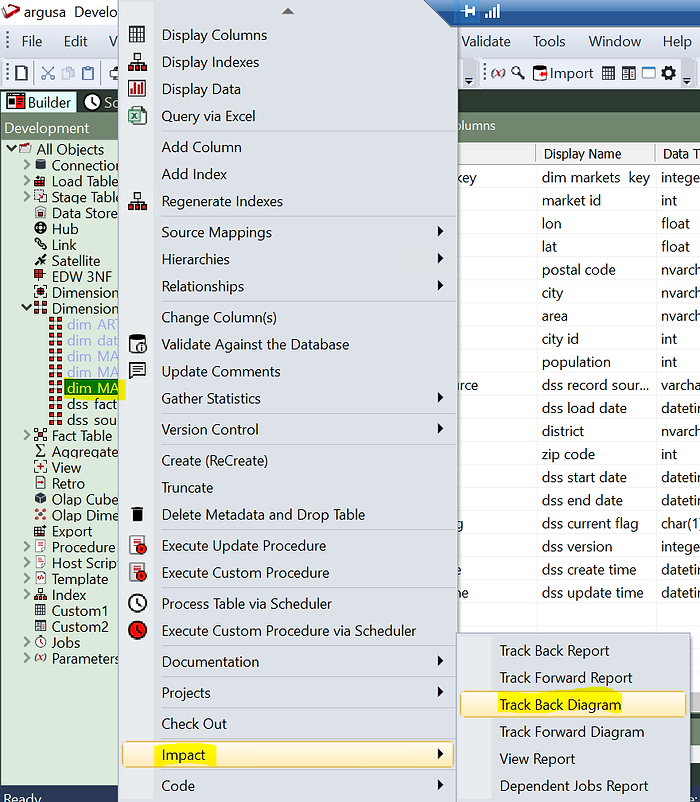
To wrap up this example we can click on the dimension and see its diagram:
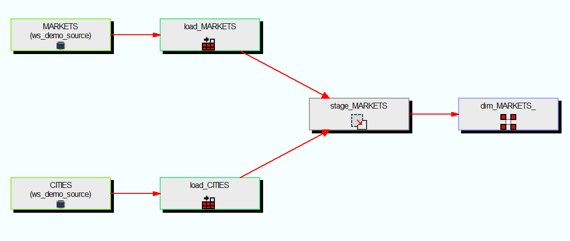
(As you can see from the diagram the stage table was not coming directly from a source table but it is a join between two source tables).
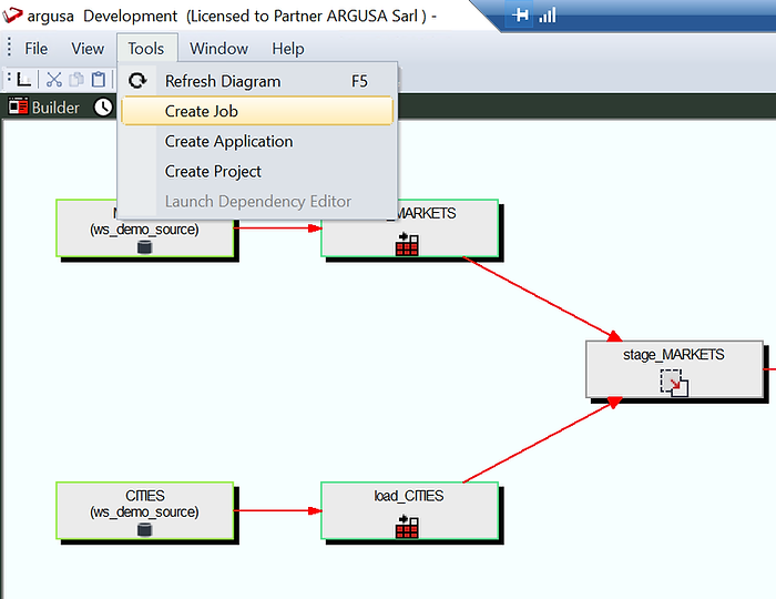
Finally, it is time to load data. We can do it very simply by creating a job from the flow diagram and running it in the scheduler.
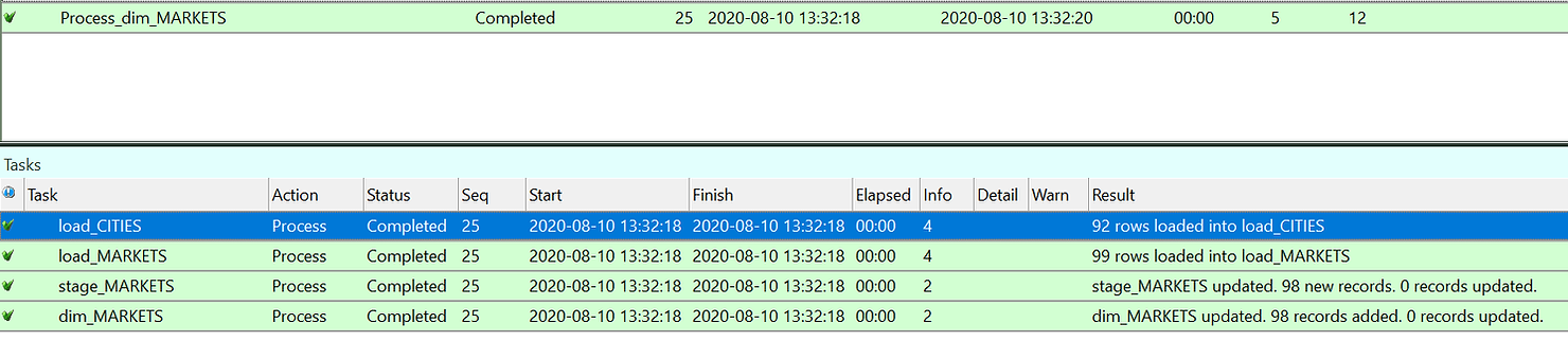
As you can see in the job log the CITIES and MARKETS tables were loaded first form the source, then the stage table was created and finally the dimensions filled.
Just as a test let’s try to run the same job again.
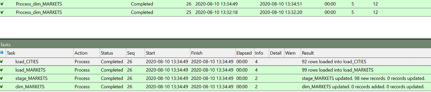
As you can see this time the first 3 steps where performed in the same way and the stage table was filled. But the data is the same, so no change was detected and therefore no update was made on the dimension table.
To wrap up let us try to modify one entry to test if our dimensions works. In particular I will change the population of a market area. To reload the data it is sufficient to click “Start Job” on the same job we have just launched to do a second run.

This time it updates one line in dim_markets. And we can also check what is the result on the table.

Two rows exist now for Kuhardt with the same market_id, the business key, but two different dim_markets_key, which is the surrogate key automatically created by WhereScape that will be used to join with the fact table. Finally, this data also includes automatically managed start and end dates and current flag for each record.
In the data warehousing world dimensional modelling is one of the simplest and most straightforward ways to present data to users. This modelling type divides data into facts, mostly quantitative data that represent measures at specific points in time, and dimensions, qualitative attributes that describe the context in which the measures are taken. For example, in the event “a car was sold in Germany for 20000 euros” the “20000 euros” is a fact and “Germany” is an attribute (therefore a dimension).
This article specifically deals with different ways to treat changing attributes with time. This might include products changing name, people changing address and so on.
The book “The data Warehouse Toolkit”, by R. Kimball and M. Ross, describes in detail eight methods to track time changes in dimensional modelling. Here we will discuss a subset of those methods, using the notation introduced by the authors in the book.
Type 0: Keep original
This method is the simplest and it is suited to treat any field with “original” (or equivalent) in its name. These values are simply not allowed to be changed. If a new value is found it is discarded and the original value is kept.
Type 1: Overwrite
This method is suited for changes that are linked to errors or for dealing with fields for which the business is not interested in tracking time changes. The method consists in overwriting the previous value. One example is customers changing birthday dates. The birthday for a person normally cannot change so we can safely assume that, if it does change, it is due to a typing mistake. For this reason, we will discard the previous birthday date and keep always the latest value. This is opposite of the type 0 approach.
Type 2: Add new row
Here we actually start tracking changes. The Type 2 method adds a new row to the dimension. New facts will be linked to the new key and old facts will keep being linked to the old key. A use case for this approach would be changing addresses. For analytical purposes, we would want to keep the address information from which each sale was made. Otherwise we might see changes in measures, e.g. delivery time, that would not be explicable if we replace the address also for old sales (which would be Type 1).
In this method some attributes need to be added on each row of the dimension. Attribute 1 and 2 are compulsory and the others are optional:
- Start date: date from which the record is valid
- End date: date up to which the record is valid
- Current flag: This flags the currently active entry, for easy filtering
- Change date: The date when the change was recorded in the data warehouse which could be different from the date that customer changed their address
- Change reason: To track which attribute on a dimension caused the creation of a new line.
Type 3: Add new column (or alternate reality)
This method is useful when a fundamental change happens in the way an attribute is defined, and the business wants to track the attribute in its old and new definition. A typical example is changes in product categorisation following a merger with another society. A TV set could be previously categorised under “electronics” and be categorised under “media” in the new company. Analysts want to be able to choose which categorisation to consider. In this case a new column is added to the dimensions mapping the old value to the new value.
Type 4: Add Mini-dimension
Sometimes in a dimension there are attributes that change at different speeds. For example, in a customer dimension, there could be the address that changes normally every few years, and the current preferred delivery method, that could change even every day as it is often modifiable with a simple click on a website. Tracking this attribute using the Type 2 approach may cause the number of rows in the dimension to grow rapidly making queries on slow changing parameters less performant. The solution is to split the customer dimension in two, each one with its own primary key in the fact table separately. One will track slow changing attributes and the other one rapidly changing ones.
Type 5: Add mini dimension and type 1 outrigger
This method is similar to Type 4 but in addition it includes the primary key of the rapidly changing dimension as a foreign key to the “main” dimension table, i.e. the table containing the slowly changing dimension. This allows to link the two dimensions directly without going through a fact table. On the other hand, the ‘main’ dimension table can only contain the “current” version of the rapidly changing attribute.
Automate it all using WhereScape
All this looks complicated to implement writing explicit SQL? There is a solution for you. Luckily these methods are based on simple rules, so they lend themselves easily to automation! WhereScape is a leader with 20 years’ experience in Data Warehouse automation. While using WhereScape, you choose the type of change tracking you want, and a wizard will help you configure the implementation without having to write a single a line of code. Furthermore, this work is easily reusable for several dimensions. In the case you want to diverge from the standard rules defined by Kimball, it is possible to edit and customise the template which generates the code, and thus automate the creation of your own change tracking algorithm.
Now, let’s see how it works. For the following example, we will suppose data is already loaded in the target database into a stage table containing markets information, including their location and characteristics.
Stage tables are working tables where transformations are done on data before loading it to the final objects (dimensions or fact tables). Typically stage tables are temporary and truncated at every load cycle. This stage table could be sourcing several source tables and already implement complex business logic. This is a good topic for another article. For now, we will focus on how to build a Type 2 Slowly Changing Dimension out of this stage table.
All we have to do is click on the “Dimension” element type in the left pane and then drag and drop the stage table into the work area.
A wizard will pop-up, helping you to configure your new dimension.
First, we need to give it a name. Notice that the wizard proposes a name for this table, following data warehouse best practices: it uses the name of the stage table and replaces “stage” with “dim”. You can of course customise the naming convention as well as a single entity name that you do not want to follow the convention. In addition, you can decide in what location to store your dimension. For example, permanently stored entities (as dimensions) are typically stored in a location with more robust backup features.
The second window asks you what kind of dimensions you want to build. As you can see Type 1, 2 and 3 are possible. You can also choose to use system generated timestamps or data driven ones. For this example, we will choose “Slowly Changing” (Type 2).
The next window will allow you to fully document your dimension, including its grain, purpose and usage. All this information will appear in the automatically produced documentation.
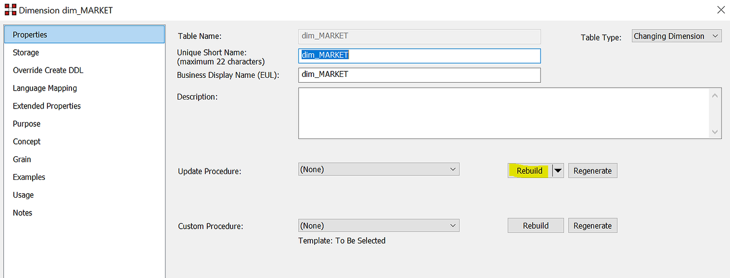
Most importantly, the wizard will build the code that will manage the inserts and updates. Modifying the DDL (data definition language) is also possible if necessary. In order to customise the update procedure, click on “Rebuild”.
In the next window you can choose to “Create” or “Create and Load”. The reason is that this might be a large table and the load can take a long time. You can therefore conveniently decide not to load the dimensions immediately after creation but later, in the background, via a scheduler.
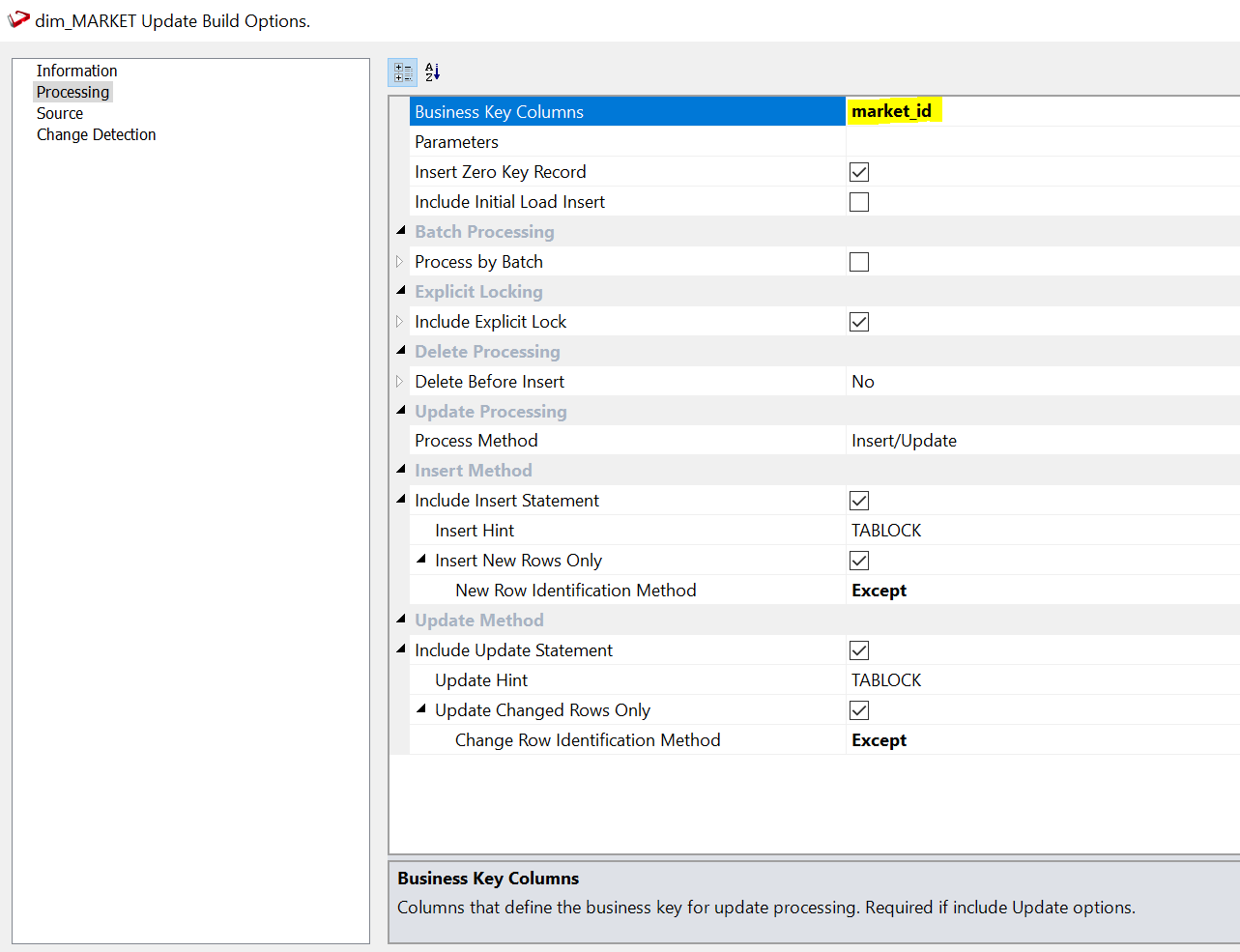
In the following window you are asked to configure the business key, i.e. the field that identifies a business element. It could be a client, a product or in this case a market. We will choose “market_id”. At the bottom of this window, you will find a helpful description of the element you are currently editing.
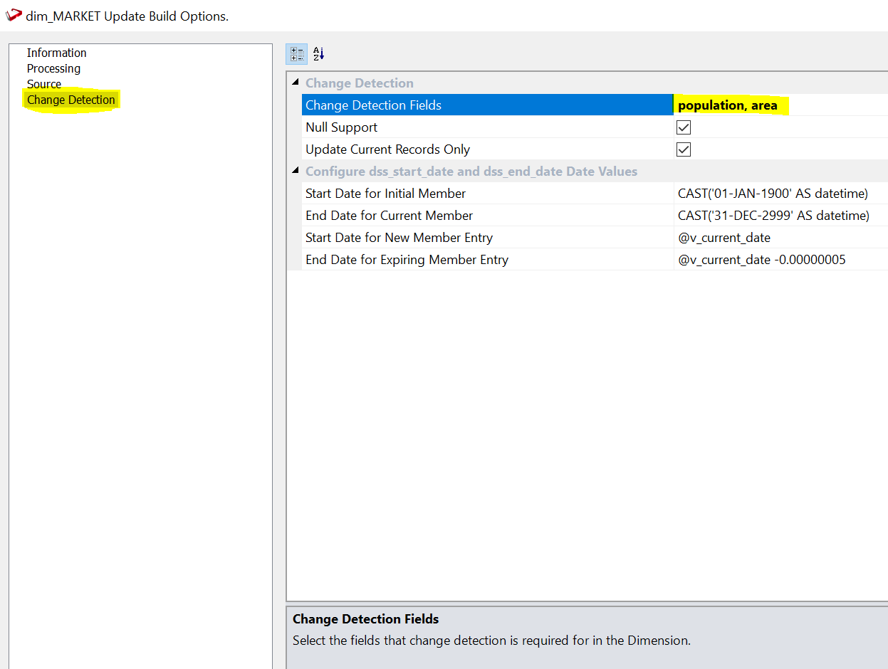
We have the possibility to setup all sorts of options, but the defaults work well in most of the use cases. The last step is deciding on which attributes we want to track change. You can do that under the “Change Detection” section.
The choice is up to you and your business representatives. For this example, we will choose population and area. A market represents a specific location, so its longitude and latitude do not change as well as the name of the city it is in. If they do change this is probably due to a mistake so we do not want to track this change in time. On the other hand, population and area are measured every year and in fast developing areas may change rapidly. And it can be interesting to keep track of how the context was when old sales were made. We will therefore track change on these two attributes.
Now we click on “OK” and our dimension is ready.
Note that a few fields were automatically created. These include the numeric surrogate key to be used as a foreign key in the fact table and all change attributes: start and end validity dates, current flag, version, first create time and last update times. As the data warehouse evolves, these fields will manage themselves thanks to the predefined update procedure that you configured using the wizard.
Looking under “Procedures” we are able to inspect the generated code and modify it, if needed. Under “Templates” it is also possible to modify the template that generates the code, in a way that all future dimensions will be built with our customisations.
WhereScape templates are comprehensive and not only handle the management of the entities, but also the logging of events and errors to keep your Data Warehouse easily under control. Rest assured that WhereScape always allows the possibility of setting up templates manually to cover exceptional use cases.
To wrap up this example we can click on the dimension and see its diagram:
(As you can see from the diagram the stage table was not coming directly from a source table but it is a join between two source tables).
Finally, it is time to load data. We can do it very simply by creating a job from the flow diagram and running it in the scheduler.
As you can see in the job log the CITIES and MARKETS tables were loaded first form the source, then the stage table was created and finally the dimensions filled.
Just as a test let’s try to run the same job again.
As you can see this time the first 3 steps where performed in the same way and the stage table was filled. But the data is the same, so no change was detected and therefore no update was made on the dimension table.
To wrap up let us try to modify one entry to test if our dimensions works. In particular I will change the population of a market area. To reload the data it is sufficient to click “Start Job” on the same job we have just launched to do a second run.
This time it updates one line in dim_markets. And we can also check what is the result on the table.
Two rows exist now for Kuhardt with the same market_id, the business key, but two different dim_markets_key, which is the surrogate key automatically created by WhereScape that will be used to join with the fact table. Finally, this data also includes automatically managed start and end dates and current flag for each record.