Previous/next row operations in Tableau

Data comes in all forms and shapes and it is often required to fetch information from different data rows to calculate indicators. This can be achieved in Tableau Desktop using table calculations.
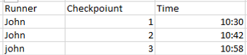
Let’s go through a practical example. We often have rows describing events in time where the timestamp on the next row represents the end time of the previous row. We can imagine a running context where a timestamp is collected when a runner reaches certain checkpoints.
To follow along you can find source files at this link, together with the solution of the proposed problems.
If we want to calculate the time interval between two checkpoints in Tableau Desktop, we can do it with the following table calculation:
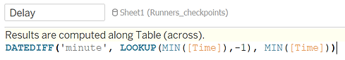
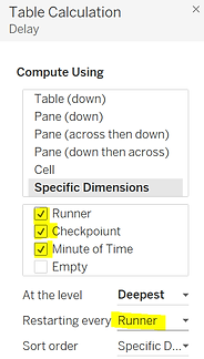
We need to perform this calculation along the checkpoint and restarting at each runner.
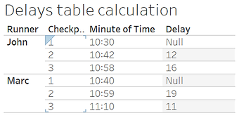
The result is the following: exactly what we needed !
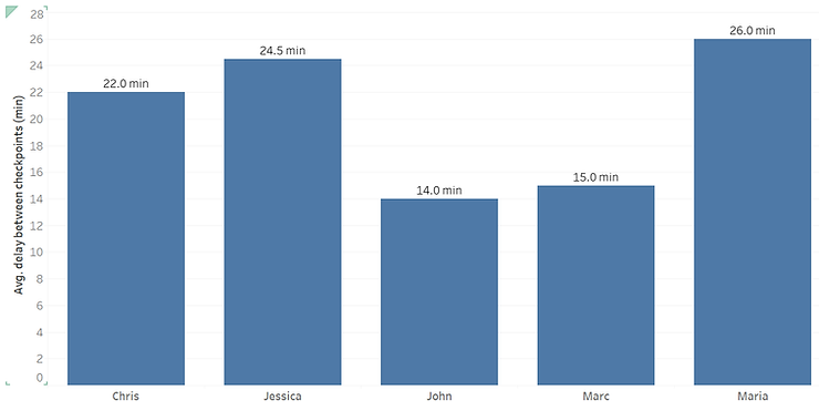
Now what if we need to calculate the average delay per runner and produce the following graph, which shows that average time a runner took, between checkpoints.
We can try to use the WINDOW_AVG function, but since these are all table calculations, we need to have the checkpoint in the view to calculate along it. Having checkpoint in the view does not produce the graph we are looking to create. One other solution could be to use some fairly complex LoD calculations, but remember that LoDs penalize performance in large datasets.
Good news ! Tableau offers a data preparation tool that could help us with this issue and allow us to Prepare the data in a format that will make the required visualization in Tableau Desktop a piece of cake. Another advantage is that this data preparation can be standardized for every user of the prepared data source.
This article demonstrates how we can fetch information for other rows in Tableau Prep.
Solution deep dive
In order to calculate the duration, we will join the table with itself, to add on each row, the timestamp of the next. To do this we need to add a key that allows us to join each row with the next.
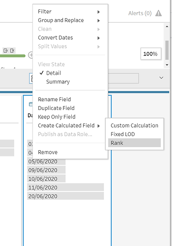
We can achieve what we want using the function rank, which can be used by clicking on the date filed and selecting « Create Calculated Field -> Rank ».
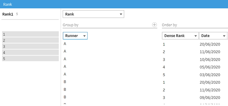
The following window opens where we can choose:
- The type of grouping if any. For example, if each row is a time measurement for a runner and we have several runners in the same table we don’t want to mix different runners’ data. We therefore need to group by the runner.
- The type of ranking. This should be « dense rank » to avoid cases where we have two times the same timestamp for a runner which would lead to duplication of rows if the two rows are given the same rank. Dense rank instead gives a different rank to each row. If their rank is the same, it just increases the rank in the order in which the rows appear.
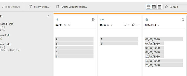
And voilà ! We now have our key, or almost. We need to join each row with the next, so we will create an order calculated field where we just add 1 to the rank.
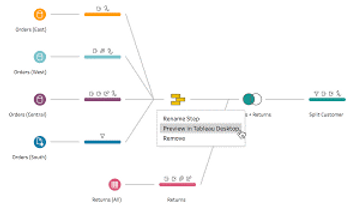
We will now proceed to create the prep flow. First, duplicate the data creating two cleaning steps on different branches. One branch will represent the core data, the second will represent the end dates. In the latter branch, we can remove all fields except the timestamp, the key and the « rank + 1 » calculation
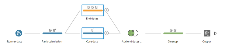
As in the “End Dates” branch we kept « Rank + 1 », we can rename the date in this branch « End Date » as it is the timestamp of the « next » row, namely the end timestamp. A similar solution could have been obtained keeping “Rank” instead of “Rank + 1” and renaming the corresponding date “Start Date”.
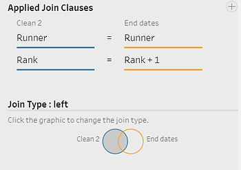
Finally, we will join the two branches on the grouping key and « rank = rank + 1 ». The type of join we chose needs close attention: this could be a left join on the core data or an inner join. If we chose a left join, we will keep all the rows from the first branch, but the first row will have no duration because it has no start date. A left join is usually what we need. We might want to only keep rows with a duration. In this case, we would choose an inner join, and the first row will be lost for each runner.
The resulting dataset contains a start date and an end date on the same row. We can now simply calculate the difference using a DATEDIFF and publish the result as a tableau data source or as a flat file.
We are now ready to plug the produced data source into Tableau Desktop and show the average delay per runner as required!
Data comes in all forms and shapes and it is often required to fetch information from different data rows to calculate indicators. This can be achieved in Tableau Desktop using table calculations.
Let’s go through a practical example. We often have rows describing events in time where the timestamp on the next row represents the end time of the previous row. We can imagine a running context where a timestamp is collected when a runner reaches certain checkpoints.
To follow along you can find source files at this link, together with the solution of the proposed problems.
If we want to calculate the time interval between two checkpoints in Tableau Desktop, we can do it with the following table calculation:
We need to perform this calculation along the checkpoint and restarting at each runner.
The result is the following: exactly what we needed !
Now what if we need to calculate the average delay per runner and produce the following graph, which shows that average time a runner took, between checkpoints.
We can try to use the WINDOW_AVG function, but since these are all table calculations, we need to have the checkpoint in the view to calculate along it. Having checkpoint in the view does not produce the graph we are looking to create. One other solution could be to use some fairly complex LoD calculations, but remember that LoDs penalize performance in large datasets.
Good news ! Tableau offers a data preparation tool that could help us with this issue and allow us to Prepare the data in a format that will make the required visualization in Tableau Desktop a piece of cake. Another advantage is that this data preparation can be standardized for every user of the prepared data source.
This article demonstrates how we can fetch information for other rows in Tableau Prep.
Solution deep dive
In order to calculate the duration, we will join the table with itself, to add on each row, the timestamp of the next. To do this we need to add a key that allows us to join each row with the next.
We can achieve what we want using the function rank, which can be used by clicking on the date filed and selecting « Create Calculated Field -> Rank ».
The following window opens where we can choose:
- The type of grouping if any. For example, if each row is a time measurement for a runner and we have several runners in the same table we don’t want to mix different runners’ data. We therefore need to group by the runner.
- The type of ranking. This should be « dense rank » to avoid cases where we have two times the same timestamp for a runner which would lead to duplication of rows if the two rows are given the same rank. Dense rank instead gives a different rank to each row. If their rank is the same, it just increases the rank in the order in which the rows appear.
And voilà ! We now have our key, or almost. We need to join each row with the next, so we will create an order calculated field where we just add 1 to the rank.
We will now proceed to create the prep flow. First, duplicate the data creating two cleaning steps on different branches. One branch will represent the core data, the second will represent the end dates. In the latter branch, we can remove all fields except the timestamp, the key and the « rank + 1 » calculation
As in the “End Dates” branch we kept « Rank + 1 », we can rename the date in this branch « End Date » as it is the timestamp of the « next » row, namely the end timestamp. A similar solution could have been obtained keeping “Rank” instead of “Rank + 1” and renaming the corresponding date “Start Date”.
Finally, we will join the two branches on the grouping key and « rank = rank + 1 ». The type of join we chose needs close attention: this could be a left join on the core data or an inner join. If we chose a left join, we will keep all the rows from the first branch, but the first row will have no duration because it has no start date. A left join is usually what we need. We might want to only keep rows with a duration. In this case, we would choose an inner join, and the first row will be lost for each runner.
The resulting dataset contains a start date and an end date on the same row. We can now simply calculate the difference using a DATEDIFF and publish the result as a tableau data source or as a flat file.
We are now ready to plug the produced data source into Tableau Desktop and show the average delay per runner as required!